
In the last two posts in this volatility series, we’ve explored some applications of the core volatility concepts that we introduced at the beginning of the series. We covered things like measuring extremes, sizing stops, choosing entries, and pricing options.
We also looked at volatility as a gauge for knowing when to be patient with positions, and when to get out (or at least get more tactical). In this post, we’ll focus specifically on this filtering application, and do some backtesting to see how effective it is in reducing risk.
Note: This post will specifically talk about a strategy you can implement, but is for educational purposes only and should not be taken as investment advice.
Why study this? Why would a volatility filter be useful?
I am not a fan of blackbox algorithms. For me, it’s crucial to understand why something works. A good backtest is just table stakes for a strategy. It’s the rationale combined with the data that should actually give you the confidence to adhere to a strategy.
When it comes to volatility in equities, especially broad market indices, what do we know to be true? We know that price velocity and volatility are pronounced to the downside. Every stock market crash is associated with expanding volatility. As the saying goes, the market takes the stairs up and the elevator down.
Now here’s the key: while volatility is mean reverting, it also has “inertia”. Technically this is called autocorrelation and it just means volatility is a predictor of itself. Volatility leads to volatility, and vice versa. Think of it like the weather. It never stays rainy or sunny forever, but often, rain follows after rain, and sunshine follows after sunshine.
All this to say, volatility is a good predictor of more volatility, and we know volatility is highly correlated with market crashes. As such, we might be able to use volatility as a key signal of when to get out of the market, thereby reducing our downside risk and reducing our portfolio volatility.
Sidebar: You don’t have to code this
Let me cover off something right quick. Below I’m going to walk through code, which is the only way to tell a computer to do it. But you can look at these things and do this strategy on your own. You can download a normalized ATR indicator I made for Thinkorswim for free here (but please consider throwing me a fiver for the effort!).
The normalized ATR parameters we use in the code below are 5 days for the lookback period, and ‘simple’ for the averaging method. When you pull up the indicator and configure it, just draw a level at the 2% line for QQQ, and you can run the strategy below manually.
Getting data
Let’s get the data and do a backtest of our volatility filter strategy using the same libraries as we did when building our All-Weather portfolio. The code here will be presented in python, using common tools for data work including pandas, numpy, and matplotlib.
First, let’s get our hands on the data
import pandas as pd
from pandas_datareader import data as web
from datetime import datetime

prices = web.DataReader(
    'QQQ', 'google', datetime(2006, 1, 3), datetime(2021, 3, 19))
Now we’ve got the daily open, high, low, close, and adjusted close for QQQ from the beginning of 2006 to mid March of 2021. This will let us calculate some volatility measures, along with the returns of QQQ.
Measuring volatility
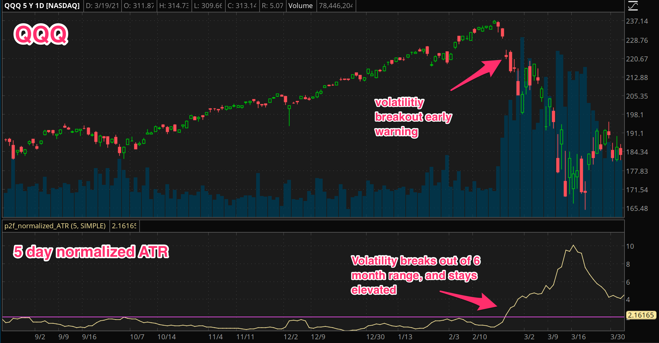
Among the volatility measures we covered in the first post of this series, we’ll use the normalized ATR here.
Why? Because the ATR incorporates the range of each day, not just the change in closing prices (like standard deviation would do). Then, normalizing it just means stating it in percentage terms. So instead of saying the daily ATR is 3.95 points, we can say the daily ATR is 2%.
For this bit, I’m skipping over the implementation of the ATR. There are a number of libraries out there, and it’s quick to code yourself by looking at the calculation. If you’re interested in reproducing these results and really just want my ATR code, shoot me an email.
We use a 5 day ATR with simple averaging, and then normalize it by dividing by the close price.
atr_data = atr(price_series, 5, 'simple')
n_atr = atr_data / price_series.shift(1)['Close'])
So if the normalized ATR is 4% for example, the value of n_atr will be 0.04.
The strategy, in English
Ok so now we have a measure of volatility, how do we use it?
Let’s revisit the premise. Crashes (big negative returns) correlate with high volatility, and volatility tends to hang around for some time once it arrives. Because, you know, people are freaking out or maybe actively trading the volatility, etc. Price discovery is happening with uncertainty.
So, for a long term strategy, we can avoid a lot of heartburn, reduce our risk, and maybe even get more returns, if we can step aside when major crashes are more likely to happen.
The trade off is that we’ll also step aside when things just look like they are crashing but don’t, and instead bounce back. We need to minimize those “false” events, and mostly try to just get out when shit is actually hitting the fan.
With the 15 year history of QQQ we have here, we want to lightly fit a parameter onto the data set, to figure out our trigger to step out.
Here I’m going to skip the speech about overfitting data. Basically, have as few parameters as possible in a strategy, and don’t try to over optimize it. Go with what fundamentally makes sense for your premise and the data set.
In this case, the normalized ATR figure we come up with as a good trade off is 2%. This is the general level of volatility that’s related to bigger falls in QQQ. Remember, this value means that over the past trading week, the average range each day (including the overnight gaps) has been 2% or bigger. Dicey!
So, our strategy is then simply: hold QQQ while the 5 day ATR is under 2%, get out when it goes over 2%.
That’s it. Could something that simple actually work? Knowing the concepts, ask yourself why shouldn’t it?
The strategy, in code
Let’s put our simple volatility filter strategy into code.
hold = (n_atr < 0.02)
sell = (n_atr >= 0.02)

units = pd.Series(data=0, index=prices.index)
units[hold] = 1
units[sell] = 0
Now we have a time series of being in or out of QQQ according to our signal. All that’s left is calculating the returns of the strategy. We’ll use the same boilerplate code from the All-Weather post.
cl = pd.DataFrame({'x': prices['Adj Close']})
weights = pd.DataFrame({'x': 1}, index=cl.index)
positions = weights.mul(units, axis=0) * cl
pnl = (positions.shift(1) * cl.pct_change()).sum(axis=1)
grossMktVal = positions.abs().sum(axis=1)

rets = (pnl / grossMktVal.shift(1)).fillna(value=0)
And now rets is the return series of the strategy.
Note that positions.shift(1) protects against look-ahead bias. It just means that we take a position at the end of the day, after we know the 5 day ATR with the current day incorporated.
Results
Let’s look at the returns for the strategy. (Click to enlarge.)
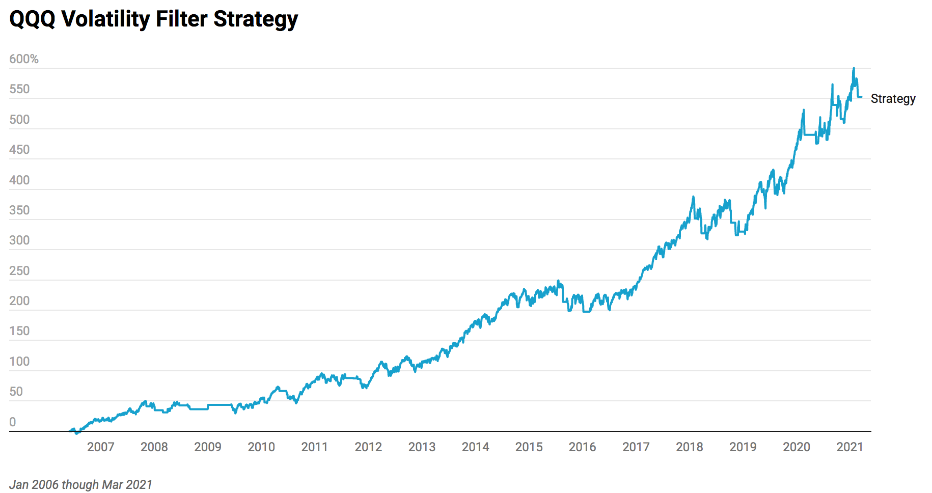
Strategy
    Total return: 5.528
    Sharpe ratio: 1.00
    APR: 0.135
    Drawdown: -0.16
    Max Time in Drawdown: 539
How do you feel about the equity curve and the drawdown? That’s often the best question to ask to evaluate a strategy. We can look at sharpe ratios, but just ask, would I trade this?
Now, let’s plot it against QQQ itself.
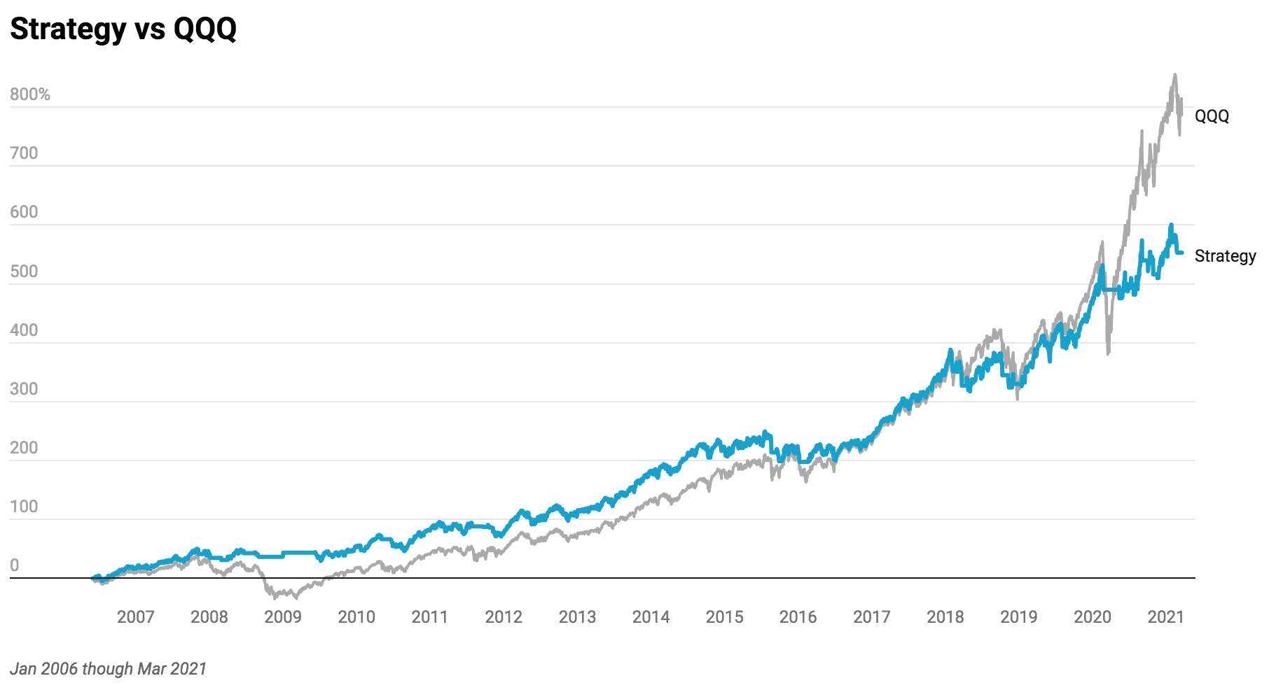
Strategy
    Total return: 5.528
    Sharpe ratio: 1.00
    APR: 0.135
    Drawdown: -0.16
    Max Time in Drawdown: 539

QQQ
    Total return: 7.896
    Sharpe ratio: 0.78
    APR: 0.159
    Drawdown: -0.53
    Max Time in Drawdown: 781
Now how do you feel about the strategy? Are we missing too much of the upside by cutting off the downside? Or is the chance at cutting out major crashes from our investing experience worth it?
There are trade offs, always. If you know what you’re doing and are comfortable with it, you can also dabble in light amounts of leverage to boost returns, which might be justified in a strategy that explicitly avoids volatility.
Don’t use leverage if you don’t know what you’re doing, ever.
For comparative analysis, let’s just take a quick look at using 25% leverage on our strategy, here again vs the QQQ.
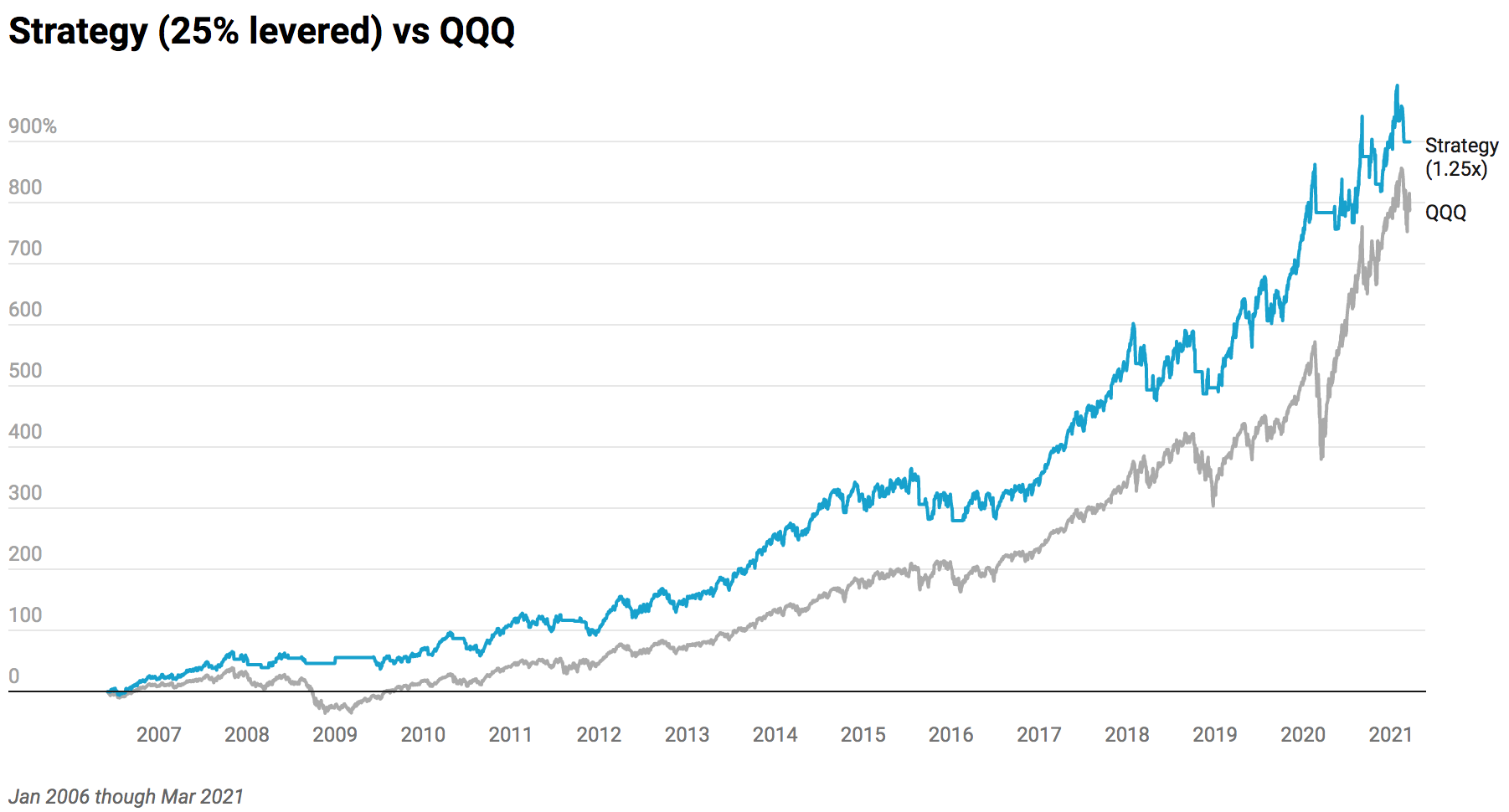
Strategy 1.25x
    Total return: 8.988
    Sharpe ratio: 1.00
    APR: 0.168
    Drawdown: -0.20
    Max Time in Drawdown: 539

QQQ
    Total return: 7.896
    Sharpe ratio: 0.78
    APR: 0.159
    Drawdown: -0.53
    Max Time in Drawdown: 781
Having better risk adjusted returns here translates to better overall returns with half the risk. Of course past performance doesn’t predict future results, etc. But the simplicity of the strategy definitely helps.
Improvements
There are some interesting ways to improve this strategy that might make sense to you. I won’t go into detail here, but one example is using a fast trend filter in conjunction with this. The idea is that, when volatility picks up, and we get out, we could miss some very big bounces that happen when the market doesn’t go all ‘global financial crisis’ on us.
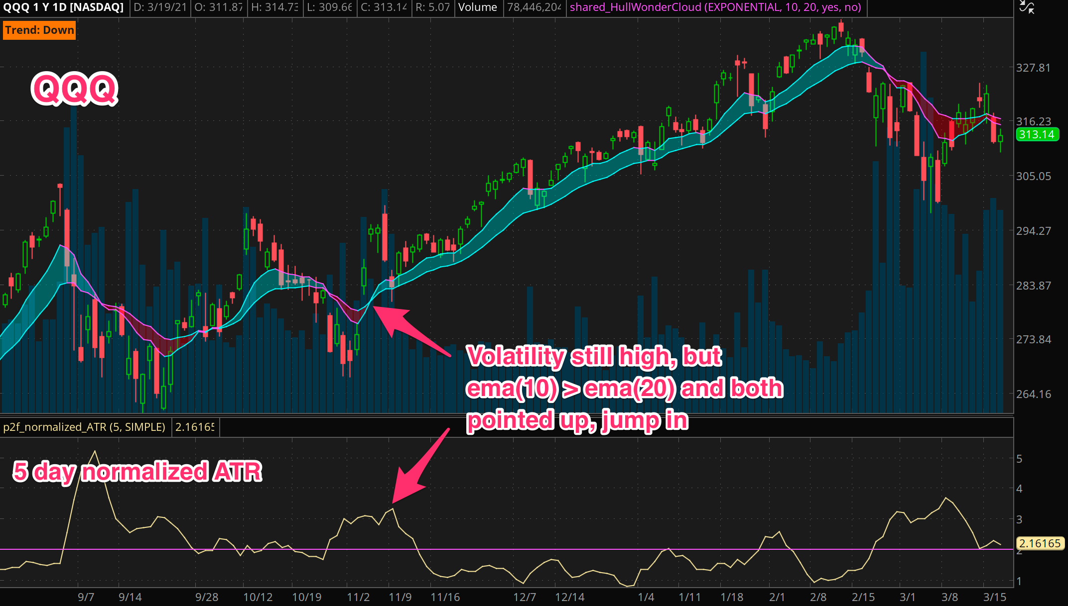
We might go over that specifically in a future post together, but I’ll leave it here for now. If you want to explore on your own, you can look at an additional rule like “get back in when ema(10) > ema(20) and both averages are moving up”. In that case the volatility could still be high, but you know the trend is pointing clearly up, so you’ve got a good chance to catch a high volatility bounce back.
Here’s a chart that shows what I’m talking about.
Onward
That wraps up this four part volatility series. I hope you were able to get value from it. (If you did, please consider making a small donation to help power this site forward.) To review, we started with volatility concepts and core measures, then looked at some of the ways they can be used, and finally ended with a specific strategy using one of those applications (“filtering”). There are many more we could explore, which might be featured in future posts here.
Hopefully this provided a practical end-to-end reference to using volatility. Should I leave you with any parting words on volatility, it is this: elevated volatility today is a good indicator that tomorrow will be volatile, and you generally should act more carefully in high volatility. Volatility has some interesting and tradable properties. Learn them, and use them!
Good trading and be smart out there!