
In our last post in the series, we saw the power of asset class diversification during good times and bad. In this post we’ll build a long-term portfolio that makes the most of the opportunity.
A little more on why
To invest real money takes some conviction. You need to see some data that supports your choices, but just as much you need to understand the basis for why it works.
This sort of diversification works because the relationships between asset classes mostly stay the same. Of course the question to ask then is why exactly do they stay the same?
This isn’t a simple answer and involves some theory around how money and assets work. Here we’ll just look at the data, but if you want to dig deeper into the why, I highly recommend this post from Ray Dalio called ‘Paradigm Shifts’.
Using data
Having some rationale to explain observed data creates true understanding, but often data is all we actually need to make predictions. In that light, with the stage set by the extra reading offered above, let’s go look at some data.
A side note: All of the code here will be presented in python, using common tools for data work including pandas, numpy, matplotlib and the like.
First, let’s round up a collection of ETFs representing some different asset classes.
tickers = [
    'SPY',  # SPDR's S&P 500
    'IWM',  # Russell 2000 small caps
    'QQQ',  # Nasdaq

    'SHY',  # iShares Short Term Govt Bonds (1-3 yr)
    'TLT',  # iShares Long Term Govt Bonds (20+ yr)  (2.6%)
    'TIP',  # iShares TIPS

    'LQD',  # Investment grade US corporate bonds
    'HYG',  # High yield "junk" US corporate bonds

    'VNQ',  # Real Estate (4.0%)
    'VEU',  # International Stocks (All world ex-US)
    'EEM',  # Emerging Markets

    'GLD',  # Gold
    'USO'   # Oil
]
This is definitely not an exhaustive list, and I don’t care to make one. This is covering some broad strokes and used to illustrate the ideas here.
Now let’s use some simple code from the pandas library to fetch daily data for these and collect them into a single universe for analysis:
import pandas as pd
from pandas_datareader import data as web
from datetime import datetime

db = {}
for ticker in tickers:
    db[ticker] = web.DataReader(ticker, 'yahoo', datetime(2006, 1, 3), datetime(2020, 7, 25))['Adj Close']
Now that we’ve got a collection of adjusted close data for the tickers above, we can analyze the relationship of their returns.
The search for uncorrelated returns
The key thesis of modern portfolio theory is that uncorrelated returns will minimize variance and lead to better risk adjusted returns for the overall portfolio.
As we saw in the last post, this idea works well for a basket of stocks, until it doesn’t. But here we’re looking at different asset classes with more persistent and fundamental relationships that shouldn’t be as subject to change.
Let’s look at the correlation of daily returns on this universe of assets. We’ll do this first by capturing the daily returns and creating a correlation matrix.
returns = pd.DataFrame(db).pct_change()
return_correlations = returns.corr()
And now, let’s look at this table, but since we’re looking for uncorrelated returns, let’s filter out every correlated pair of assets (i.e. ignore those pairs with correlation of returns higher than 0.2):
return_correlations[return_correlations < 0.2].fillna('')*Click the image for a closer look.
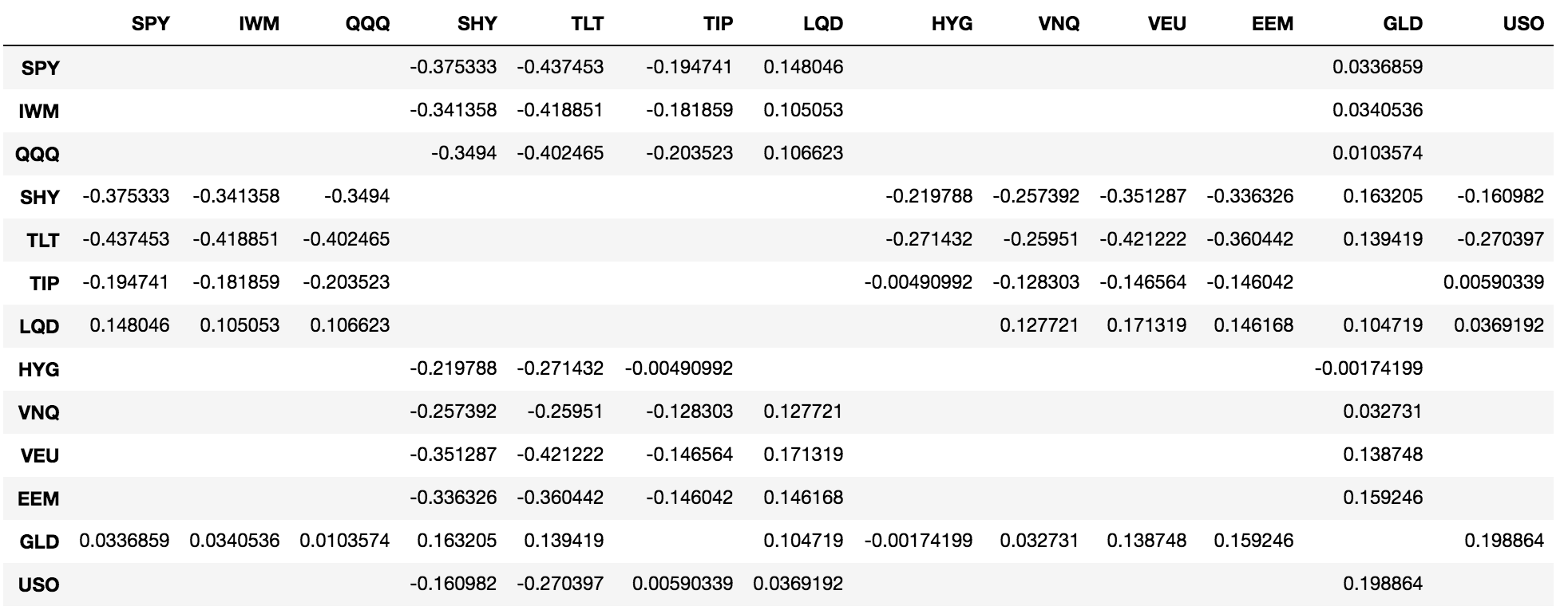
As you look at any particular column, you can scan down to the correlation of that ETF with the others. Many, like TLT for SPY, exhibit a pretty strong negative correlation. Others like GLD, are just marching to the beat of their own drum altogether.
What we find in looking for uncorrelated returns is that there are really two primary groups of assets - equities and debt instruments. All the indices correlate to each other, and the same with most of the debt instruments. It’s interesting to note though that high yield corporate debt is more correlated to equities than other debt instruments. And notably, gold stands out as another class that’s uncorrelated to both equities and debt.
A dead simple portfolio
So, using these results as a guide, let’s put together the simplest portfolio that takes advantage of noncorrelation.
Now, there is some math from modern portfolio theory we could apply here, which would tell us, based on history, the most optimal mix of assets to minimize variance and maximize returns, but… let’s avoid overfitting the data, and more importantly just keep it simple.
Instead, let’s just take a little bit of each major category, and make our portfolio like so:
- SPY - Large cap U.S. equities - 40%
- TLT - Long term U.S. government debt - 40%
- GLD - Gold - 20%
This should give us good exposure to the major asset categories, along with some secondary exposure to a third category that will help further minimize volatility in our portfolio and smooth out returns.
The magic of rebalancing
A key element in this type of portfolio is regular rebalancing.
For one, it’s necessary to do in order to keep the same overall effect of uncorrelated returns. If we never rebalanced and one asset rose while the others fell, it would start to have an oversized weight on the overall returns of the portfolio. We then start losing the benefit of minimizing variance and getting better risk adjusted returns.
But the other benefit of rebalancing is the routine of buying low and selling high. When you manage a portfolio like this, you’ll find yourself quite happy on days when different markets go to extremes.
During market crashes when equities are crashing, you’ll often find bonds and gold racing higher. At that moment, you get the opportunity to sell fear assets at their highs, while buying up equities as they go on sale. The overall effect means you’ll start accumulating more and more shares of all the asset classes over time, as you get new opportunities to fund purchases with proceeds from your outperformers.
Reviewing results
Let’s take a look at how our simple portfolio above performed starting from 2006 to now. This takes us through both the global financial crisis of 2008 and 2009, as well as through a 10 year bull market in equities, and a couple key drops in 2018 and 2020.
First, let’s work out a quick bit of code to model the 40% / 40% / 20% portfolio and then compare the cumulative returns of it against each of the individual assets.
def cumret(ret):
    return (1 + ret).cumprod() - 1

portfolio_returns = \
    (db['SPY'].pct_change() * 0.4) + \
    (db['TLT'].pct_change() * 0.4) + \
    (db['GLD'].pct_change() * 0.2)

pd.concat([
        cumret(rets),
        cumret(db['SPY'].pct_change()),
        cumret(db['TLT'].pct_change()),
        cumret(db['GLD'].pct_change())],
    axis=1,
    keys=['Portfolio', 'SPY', 'TLT', 'GLD'])
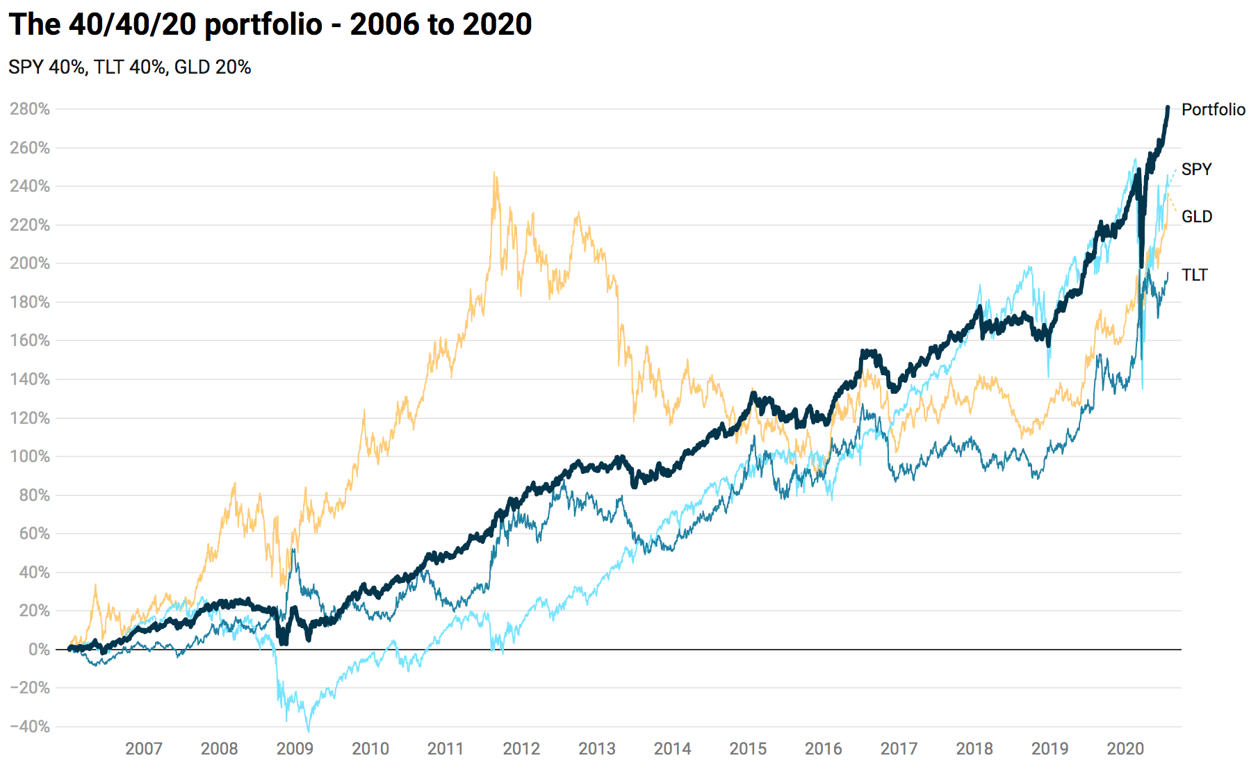
What you’ll see is a much steadier equity curve from the portfolio than any of the underlying assets. Seeing the results plotted together helps visually explain why. This can be seen most clearly in the 2008 through 2009 period, as SPY dropped almost 60% from it’s high water mark. First gold began to save the portfolio as stocks made a slide from these highs, and then bonds spiked as stocks went into an all-out crash.
These inverse returns don’t just happen during extreme events either, they tend to move independently or oppositely day in and day out, leading to a portfolio that rarely experiences major volatility, but continues to rise as global capital markets realize continued productivity gains in the world.
Below are some high level measures of performance for this portfolio and SPY. Take particular note of the difference in sharpe ratio:
SPY
        Total return: 2.397
        Sharpe ratio: 0.52
        APR: 0.088
        Drawdown: -0.55
        Max Time in Drawdown: 1223

Portfolio
        Total return: 2.808
        Sharpe ratio: 1.07
        APR: 0.096
        Drawdown: -0.19
        Max Time in Drawdown: 333
Not only is the portfolio beating the market with higher annual returns across this 14 year period, it’s doing so with much less risk, represented here with the sharpe ratio and supported by the drawdown figures.
In terms of drawdowns, while equity only portfolios had to wait over 1223 trading days, or 5 years, to get even again after the GFC, this balanced portfolio had less than 20% drawdown and bounced back to even in just 18 months.
Implementing and managing
The all weather portfolio I run today looks very much like the one covered here, with a few tweaks inside of those major categories of equities, debt, and inflation hedges (discussed here as gold).
Think of this as a framework that promotes portfolio stability while still affording you the opportunity to seek over-performance within a category, by picking individual names or instruments.
But you can absolutely run your a portfolio just using the ETFs given above, and I still run at least one portfolio which follows exactly as outlined here.
Implementing this yourself is pretty simple. For example, if you have $10,000 to invest, open an account with online broker like E-Trade or TDAmeritrade, and buy $4,000 dollars worth of SPY, $4,000 worth of TLT, and $2,000 of GLD. As time passes and these move around, you’ll find that you start to drift from 40%, 40%, 20% allocations.
To rebalance, just calculate what 40% or 20% of your portfolio value is today. Look at that number versus your actual position size and buy or sell to realign.
For example, if your portfolio value has grown from $10,000 to $11,000, you want your SPY position to be $11,000 * 40% = $4,400. But you might discover that it has grown to be a $4,750 position instead. In that case, you just need to sell $350 dollars worth of shares. Then do the same for TLT and GLD.
You can choose to rebalance any time you want, including every month, every 6 months, after a certain amount of drift, or maybe even just when major moves in these markets happen and you want to take advantage of them.
And on we go…
Hopefully this series has helped explain a simple but powerful way to invest for the long haul, and how to reassess that process over time.
Uncorrelated returns help create stability, and if we can find stable relationships of noncorrelation, we can translate it into solid returns.
One topic we didn’t touch on at all, but is quite relevant here, is what extent leverage can be applied to this type of portfolio. Since drawdowns are historically well protected by the inverse correlation of returns, it is possible (though not necessary) to lever up the portfolio and squeeze a bit more out of it.
Alas, I leave that to you to consider, along with this framework for creating portfolios that stand a better chance of weathering the many storms yet to come.