
Volatility is a fundamental concept that informs every trader and investor in one way or another. As we saw in the All Weather Portfolio series, which focused on minimizing volatility through diversification, the concept has application even in long-term passive investing. By building a solid understanding, we can find new ways to put volatility to use for short and long term gains.
In this series of posts, we’ll introduce some core concepts and measures of volatility, look at a set of applications for those concepts, and wrap it up by building a simple trading strategy that uses volatility (and beats the market).
Volatility Intuition: Movement and Spread
One basic way to describe volatility is as the magnitude of uncertainty. We can look outside the world of finance and get a grasp on it. For example, if you describe a person as volatile, they might have serious mood swings and unpredictable behavior. If you describe a substance as volatile, it could cause harm without much warning. If the conditions out at sea are volatile, they are going to be very choppy and dynamic.
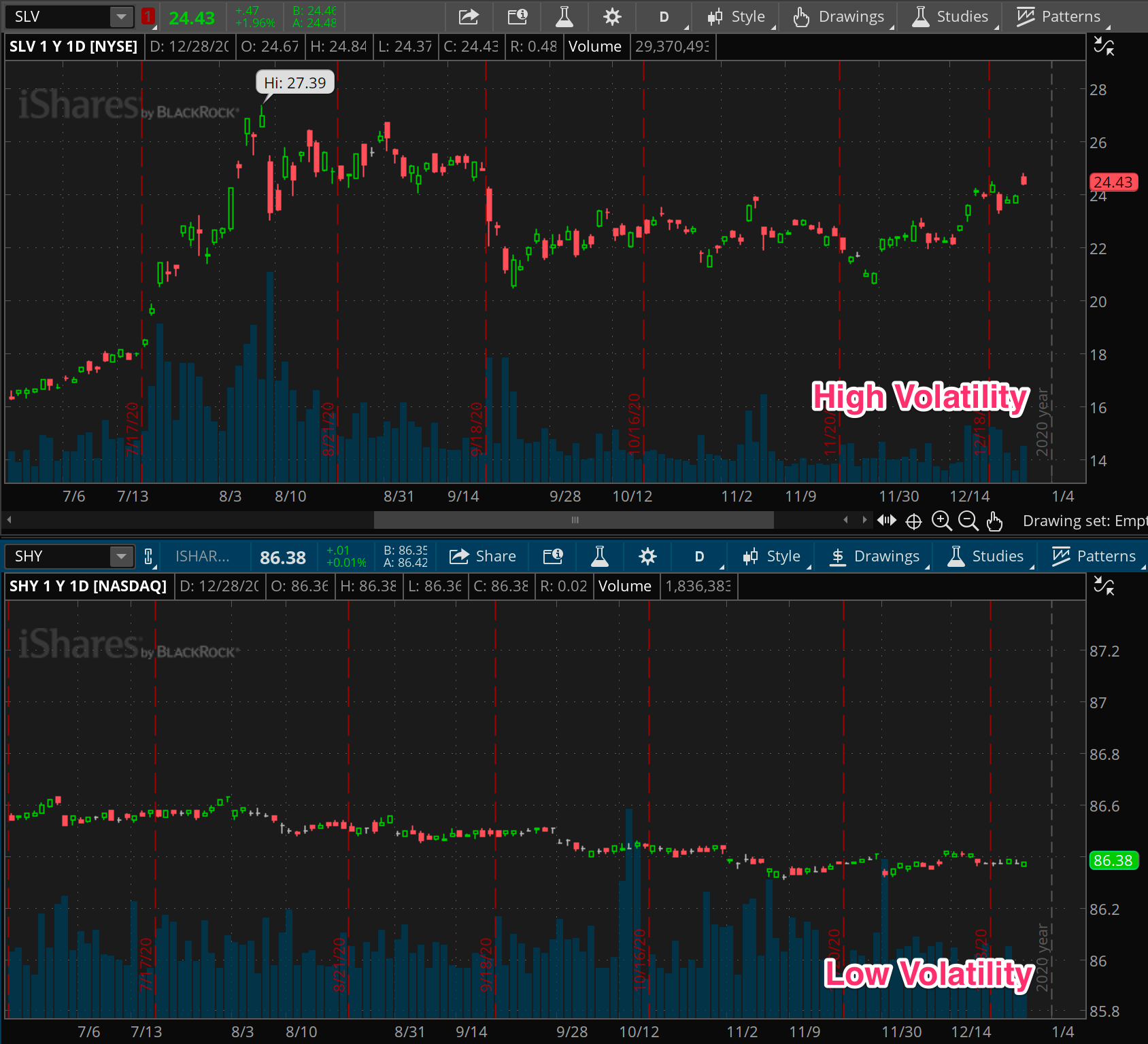
In every case, there’s a marked uncertainty in outcomes. Volatility is the opposite of calm, steady, certain, or predictable. This applies to markets as well. Measures of volatility in the market capture a range of movement. Higher volatility indicates a wider range of price movement, while lower volatility indicates a smaller range. And when the range is large, there is less certainty about where the price will end up next. That is the essence of it and the key to understanding volatility.
How do we measure this range of movement in a way that is mathematically defined, consistent, and useful? In this post, we’ll go over a few core measures of volatility.
Standard Deviation
This is the reference measure for volatility, and it comes right out of the statistics books. It’s defined as the square root of the average of squared differences between prices and the moving average of price. Makes perfect sense right?
Ok, let’s take a step back and break it down. By that I don’t mean digging into the equation and showing you an excel sheet; others can do that just fine. I mean let’s break down the concept into something that makes intuitive sense.
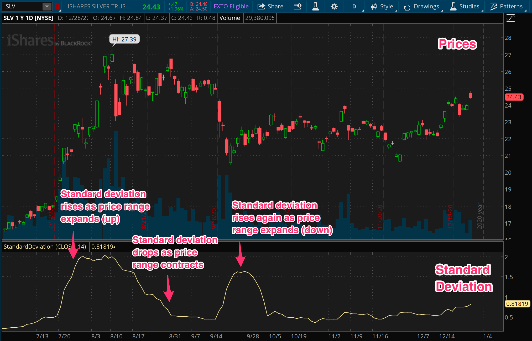
Remember, all we’re after here is a measure of range, or in other words, the amount by which prices are spread around some baseline. In our case, the baseline is a moving average of prices, and represents where price should stay if nothing is happening. The standard deviation gives us an average distance of prices around that baseline.
So then, the wider the distance of prices from that average, the greater the standard deviation. Conversely, the more that prices are tightly clustered around an average, the smaller the spread of prices, the lower the differences, and the smaller the standard deviation.
What makes standard deviation such a valuable measure is just how much research and understanding has been built up around the concept. In the distributions of many random variables (such as price returns), the standard deviation is defined such that around 67% of future random values ought to fall within one standard deviation above or below the average. An impressive 95% of values should fall within two standard deviations above or below the average.
Alas, like everything in the markets, both the average and the standard deviation itself are dynamic and subject to change. That’s why we always consider them on a rolling basis, looking at the moving average and the moving standard deviation.
Average True Range
While the standard deviation measure has some strong grounding from statistical research, it’s not the only game in town. There’s also an incredibly popular measure among traders and market researchers called the Average True Range, or ATR.
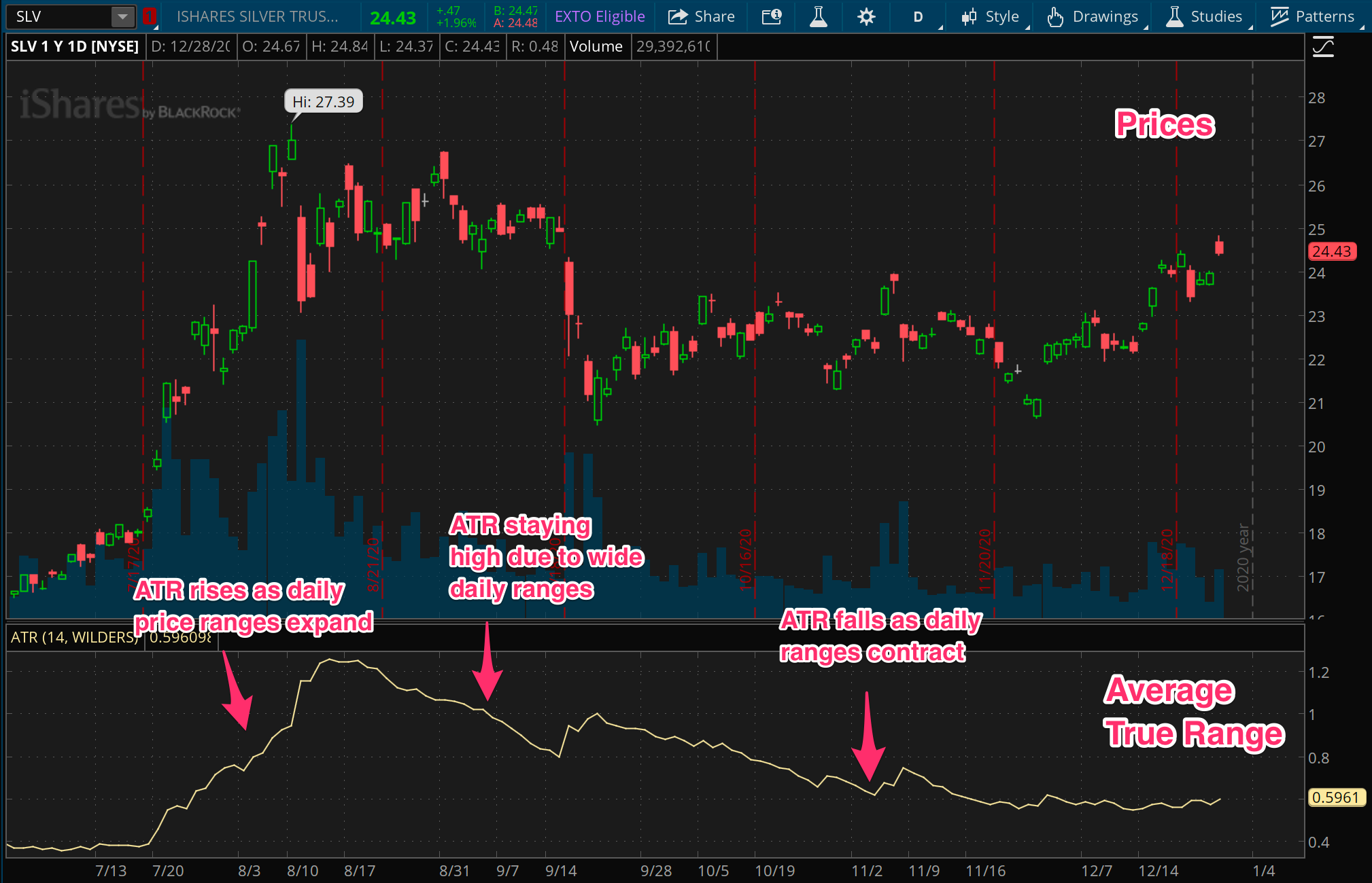
The definition of ATR goes like this: First, you need to calculate a “true range” for each period. Then just average them up. The true range for any given period is going to be the difference between the high and low for that period, except if the prior period’s closing price is outside of that range. Then it’s the difference between the high or low and that prior closing price. So basically, each true range value might use the prior period to account for gaps.
One of the key differences between standard deviation and ATR is that the standard deviation focuses on a series of single data points for the input (closing prices), while ATR considers a series of multiple data points (high, low, and prior close). In this way, if you consider that each period has its own range, ATR is incorporating all of those ranges into the measurement of price spread, instead of just the final closing price in each period.
This difference means that standard deviation can be understated vs ATR in many cases. Imagine the extreme case where price is swinging around a huge range each day but happens to be closing around the same price at the end of the session. The standard deviation of daily prices will be small since there’s not a large difference in each closing price and the average closing price. However the ATR will account for the highs and lows along the way as well, and be much larger than the standard deviation.
Implied Volatility
For fear of opening a Pandora’s box of option concepts, let’s take a quick detour and discuss implied volatility for a moment.
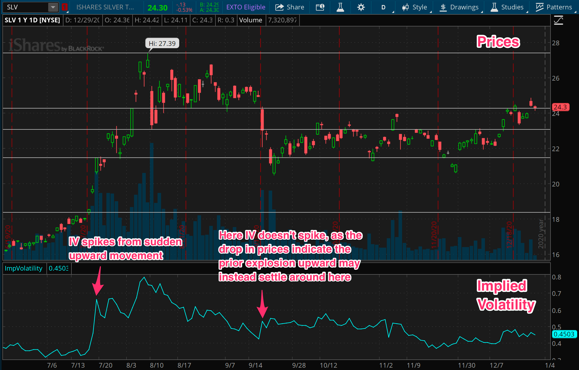
The measures we’ve covered so far pertain to realized volatility. Like most every other measure of prices, they are based on what has happened in the past. But implied volatility, or IV, is a different beast altogether. It’s a forward looking measure based on the options market associated with the instrument.
The essence of it is this: theoretically, options are made to work a bit like insurance. An option buyer pays something like an insurance premium in order to get paid out under certain circumstances (i.e. price movements), while someone else collects that premium in exchange for having to pay out the buyer under certain circumstances. While there are a lot of different options and option spreads, the easiest example to think of is a put option, which pays the buyer if the instrument’s price moves under the option’s strike price. The buyer pays a premium for this downside protection, while the seller collects the premium and promises to pay if the instrument’s price falls under the strike price.
Like everything with a market, the price of this premium moves around. Let’s stop and consider why. As with all markets, demand will move prices higher. But what drives that demand? Anticipation, fear, information… expectations. When the premium is high, it implies an expectation that the underlying instrument could move further and faster than when the premium is low. This expectation of movement, based on option premiums, is measured as the implied volatility of the underlying.
The landmark measure of implied volatility in the broad U.S. market is the VIX, which is based on the price of option premiums for the S&P 500 index. When the VIX is high, it implies an expectation that the market will be volatile, and when it’s low, it implies an expectation that the market will be calm. But any instrument out there with an option market (and there are many) will have an implied volatility according to the option prices in that market.
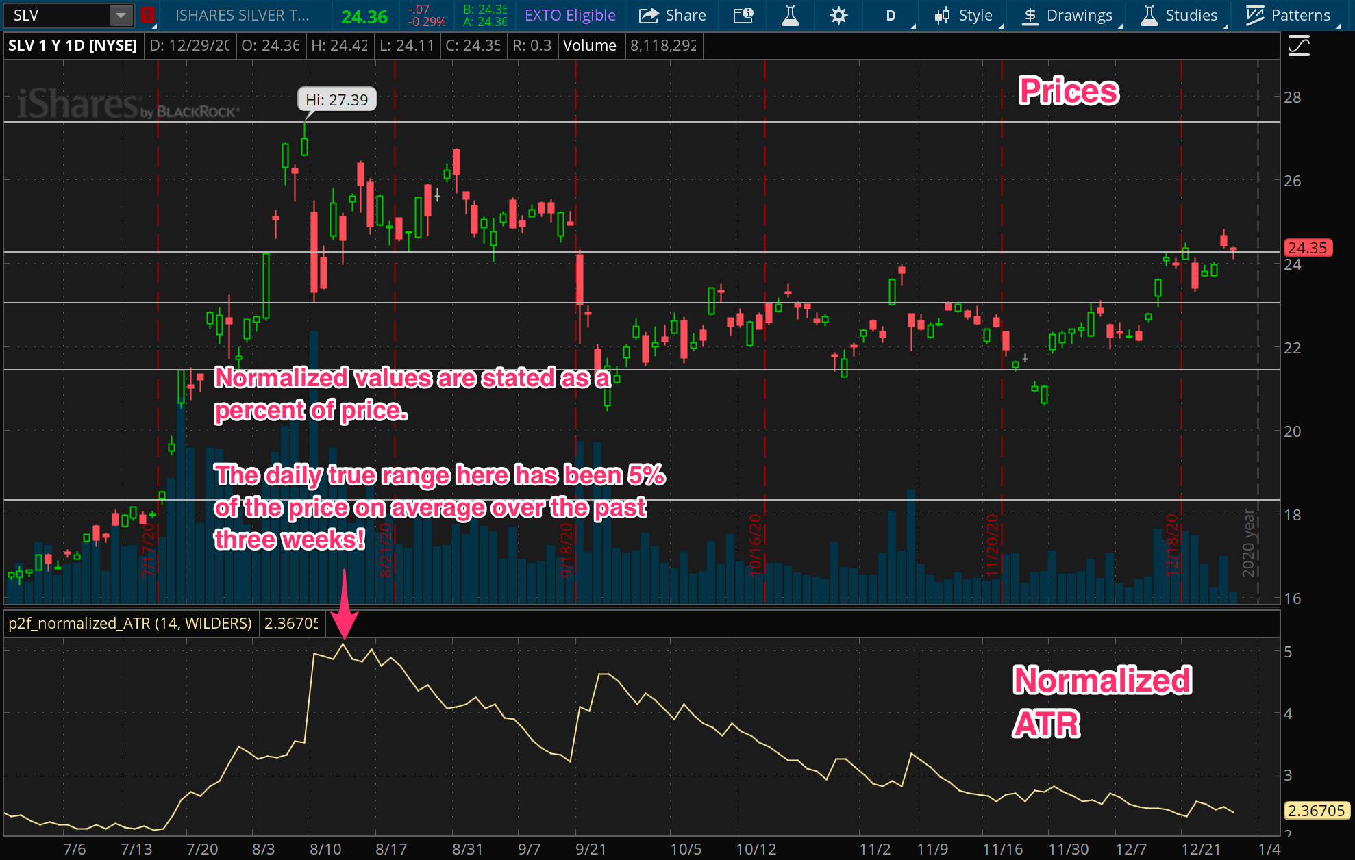
Normalized measures
In wrapping up this post on core volatility measures, let’s finally talk about normalizing. Despite the name, this has nothing to do with putting these measures through therapy or rehab. Simply put, this is just a matter of stating things as percentages rather than base values. This is done by dividing the base value of the measure by the current price.
Now, why would you ever want to do that? After all, if you’re looking at AAPL and observing its volatility, you might just want to know it’s been moving around in a $2 range every day for the past week. If you’re setting a stop of 3 times ATR for example, you’ll want to know how far away that is in price, not percentage.
For scenarios like that, the base values will always be relevant. But the key drawback with the base value is that its meaning is relative to the current price. A daily range of $2 on a $10 stock is very different from a daily range of $2 on a $100 stock. The key upside with normalized measures is that they can be compared across instruments and across time.
That ability to compare different instruments and different time periods can be crucial in building algorithms and backtesting. Because stocks generally rise over time, any base value measures will rise over time as well. In our example above, the $10 stock and the $100 stock might very well be the same stock, just at different times. The normalized measures will let us have a single universal range (0 - 100%) to observe the volatility of any instrument at any point in time.
Follow these links for normalized ATR and normalized standard deviation indicators for I built for Thinkorswim, free of charge. (Though if you appreciate using them, consider making a small donation for this site.)
How to use volatility
In this post, we introduced a few core measures of volatility. In the next post in this series, we’ll go through some applications of these measures. There are many places where volatility proves useful, and it plays a crucial role in many trading strategies. Whether as a filter, a signal, a stop, for position sizing, or some other purpose, volatility tends to show up everywhere in trading.